4 cardinalR: Generating Interesting High-Dimensional Data Structures
Simulated high dimensional data is useful for testing, validating, and improving algorithms used in dimension reduction, supervised, and unsupervised learning. High-dimensional data are characterized by multiple variables that are dependent or associated in some way, such as linear, nonlinear, clustering, or anomalies. Here, we provide new methods for generating a variety of high-dimensional structures using mathematical functions and statistical distributions organized into the R package cardinalR. Several example data sets are also provided. These will be useful for researchers to better understand how different analytical methods work and can be improved, with a special focus on nonlinear dimension reduction methods. This package enriches the existing toolset of benchmark datasets for evaluating algorithms.
4.1 Introduction
Generating synthetic datasets with clearly defined geometric properties is useful for evaluating and benchmarking algorithms in various fields, such as machine learning, data mining, and computational biology. Researchers often need to generate data with specific dimensions, noise characteristics, and complex underlying structures to test the performance and robustness of their methods. There are numerous packages available in R for generating synthetic data, each designed with unique characteristics and focus areas. The geozoo package (Schloerke 2016) provides functions to generate standard high-dimensional data like cubes, spheres, and simplexes, along with some prepared datasets. The snedata package (Melville 2025) provides functions for generating common examples used in dimension reduction publications and to download benchmark data sets. The splatter package (Zappia et al. 2017) is designed to simulate complex biological data, capturing field-specific nuances such as batch effects and differential expression. The mlbench package (Leisch and Dimitriadou 2024) provides access to benchmark datasets commonly associated with established classification or regression challenges. The surreal package (Balamuta 2024) implements the “Residual (Sur)Realism” algorithm (Stefanski 2007) to generate datasets that embed hidden images or text into residual plots, providing engaging visual demonstrations for teaching model diagnostics. Beyond R packages, other approaches include simulation frameworks based on finite mixture models (Maitra and Melnykov 2010) and evolutionary methods such as HAWKS (Shand et al. 2021), which generate challenging clustering benchmarks by optimizing dataset difficulty.
The current work implemented in the cardinalR R package builds on these approaches. It provides functions to generate a more extensive set of high-dimensional data structures, allowing users to: (i) construct high-dimensional datasets based on geometric shapes, including the option to enhance dimensionality by adding controlled noise dimensions; (ii) introduce adjustable levels of background noise to these structures; and (iii) combine the shapes to produce multiple clusters. The user can control characteristics such as the number of dimensions, shape, and sample size. It is designed to provide researchers with synthetic datasets to evaluate the performance and interpret the fit of NLDR methods, clustering algorithms, and visualization techniques. These datasets can also serve as benchmark examples for exploring how different choices of algorithm parameters affect the identification or representation of cluster and manifold structures in high-dimensional spaces.
The motivation for developing this package originated from our own work in studying nonlinear dimension reduction (NLDR) algorithms. We wanted to conduct a visualization experiment to understand the perception and misperception of a variety of NLDR methods. This required simulated datasets with carefully controlled geometric and clustering properties. While some existing packages provided useful starting points, none fully supported the creation of flexible, high-dimensional data with the specific structural variations needed for our experiment. Developing these generators for research purposes underlies cardinalR, which is now a general-purpose package that should be useful for research and teaching.
The example data structures are best viewed using a tour (Asimov 1985). These show the data as a sequence of low-dimensional projections (typically 2\text{-}D), providing a good sense of the shape in high dimensions. The interactive tour plots included in this chapter are produced using the software langevitour (Harrison 2023).
The next section provides an overview of the usage of the cardinalR package, illustrating how its modular components can be combined to generate complex high-dimensional datasets. This is followed by a section describing the implementation of the package, including its design principles and key functions. The Application section then demonstrates how the simulated clustering structures can be used to evaluate and compare dimension reduction and clustering methods. Finally, we give a brief conclusion of the chapter and discuss potential opportunities for the use of our data collection.
4.2 Usage
The cardinalR package is built on a modular framework where individual geometric generators (e.g., Gaussian, cone, sphere) create well-defined shapes (A full list of shape generators is available at https://jayanilakshika.github.io/cardinalR/reference/index.html.), which can then be combined into a single dataset including scaling, rotation, and translation. The package is available on CRAN, and the source is available on GitHub at https://github.com/JayaniLakshika/cardinalR.
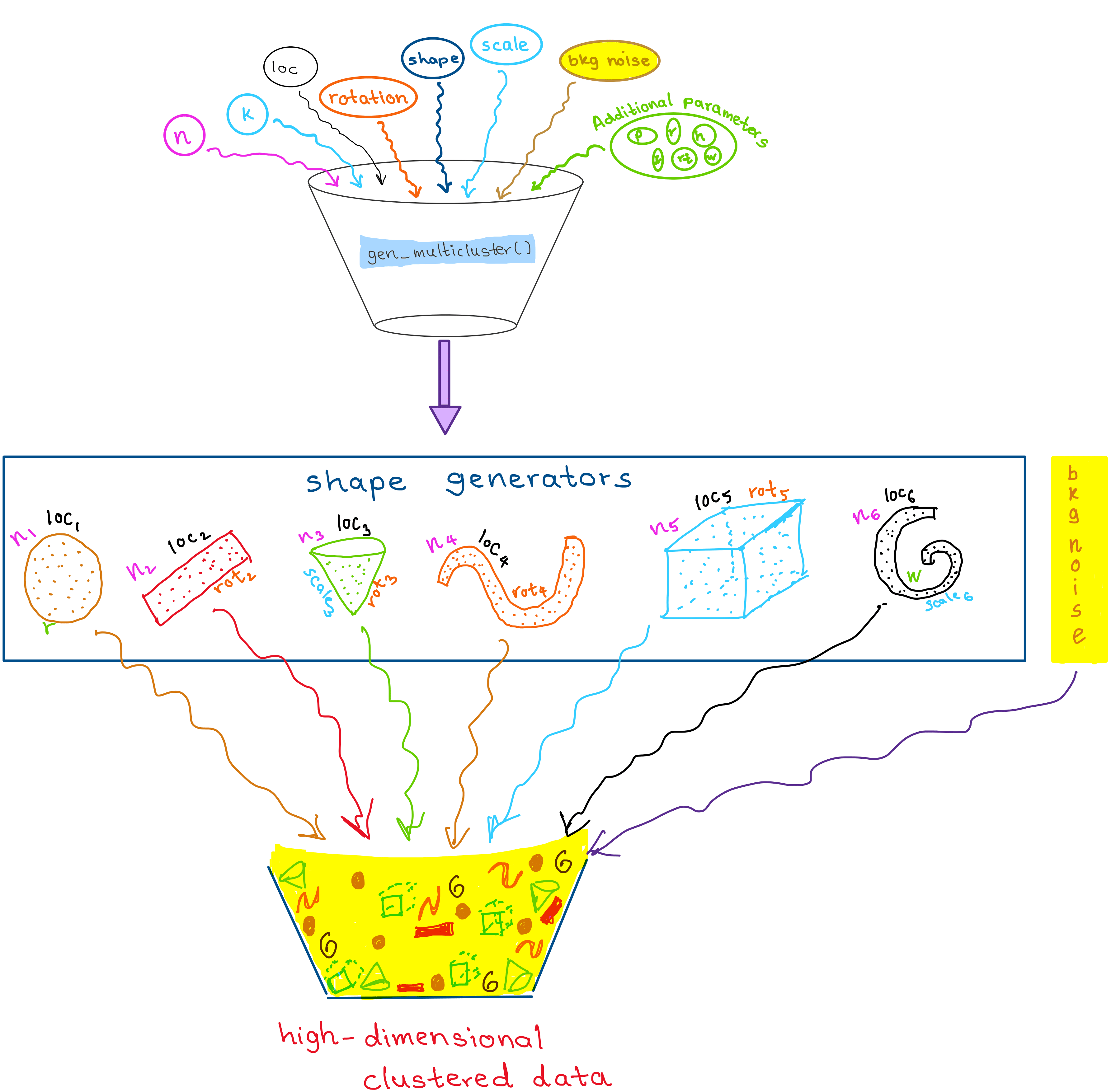
The main function, gen_multicluster(), is an all-in-one function that includes generating individual shapes, handling scaling and rotating of these shapes, and combining the result into a single unified dataset. This function and associated workflow allow flexible construction of complex, high-dimensional structures for evaluating clustering and dimension reduction methods. Figure 4.1 illustrates the workflow of gen_multicluster().
Users can control the number of clusters (k) and the number of points in each cluster (n). Each cluster can take on a different geometric shape (e.g., Gaussian, cone, uniform cube) by specifying the corresponding generator function (shape), can be scaled to adjust its spread, rotated using custom rotation matrices (rotation), and positioned at defined centroids (loc). The function ensures flexibility in cluster location and orientation, allowing users to simulate complex high-dimensional structures.
The following is an example of a three-shape multiclustered dataset. The first shape is Gaussian, the second conical, and the third a cube.
Here, the shapes have 200, 300, and 500 points respectively (n), are positioned in 4\text{-}D space according to a location matrix, loc, and stretched according to the scale. The details of the individual shape generators and the noise elements are contained in the following sections.
4.3 Implementation
The main function of the package is gen_multicluster(), which generates datasets consisting of multiple clusters with user-specified characteristics. To maintain consistency across generators, the function identifies the arguments required by each chosen generator function and supplies only those arguments that are valid for that specific generator. This design enables the combination of cluster types with differing parameter requirements within the same dataset. When clusters are generated with fewer dimensions than others, the function augments the lower-dimensional clusters with additional Gaussian noise variables so that all clusters are represented in the same dimensional space. These noise dimensions are drawn independently from normal distributions X \sim \mathcal{N}(\mu, \sigma^2), where the mean (\mu) is set to the average of the cluster coordinates and the standard deviation (\sigma) defaults to 0.2.
An optional argument, is_bkg, controls the inclusion of background noise in the dataset. When this option is set to TRUE, additional points are generated from a multivariate normal distribution with mean equal to the overall centroid of the dataset and covariance matrix. This covariance matrix is defined as diagonal, with each diagonal element corresponding to the empirical variance of the respective dimension across all clusters, ensuring that the noise reflects the overall spread of the data while remaining uncorrelated across dimensions. These background points are not assigned to any cluster and introduce low-density regions between and around clusters.
Extra arguments (...) can be passed to the cluster generating functions, allowing further control over per cluster characteristics, such as the radius of a spherical cluster. The main arguments of the gen_multicluster() function are summarized in Table 4.1.
gen_multicluster().
| Argument | Type | Explanation |
|---|---|---|
n |
integer (vector) | Number of points in each cluster. |
k |
integer | Number of clusters. |
loc |
numeric (matrix) | Locations/centroids of clusters. |
scale |
numeric (vector) | Scaling factors of clusters. |
shape |
character (vector) | Shapes of clusters. |
rotation |
list of numeric matrices | Rotation matrices, one per cluster. |
is_bkg |
logical | Background noise should exist or not. |
Shape generators
The shape generators form the foundation of the package, providing functions to create synthetic datasets from simple, well-defined geometric forms such as cones, pyramids, spheres, grids, and branching structures. Each generator includes the parameter n, which specifies the number of points to generate. Some functions, such as gen_unifcube(), also take the dimension p, while others include arguments specific to the geometry (e.g., radius for spheres (r), width for bands (w)). If higher-dimensional data are required, additional noise dimensions can be appended after data generation using any noise generator function. This flexibility allows users to construct both low- and high-dimensional datasets from the same underlying structures. Table 4.2 outlines these functions. The main arguments of the functions described in Table 4.3.
| Function | Arguments | Explanation |
|---|---|---|
gen_expbranches |
n, k |
Exponential shaped branches. |
gen_linearbranches |
n, k |
Linear shaped branches. |
gen_curvybranches |
n, k |
Curvy shaped branches. |
gen_orglinearbranches |
n, p, k |
Linear-shaped branches originated from one point. |
gen_orgcurvybranches |
n, p, k |
Curvy shaped branches originated from one point. |
gen_cone |
n, p, h, ratio |
Cone-shaped structure. |
gen_gridcube |
n, p |
Cube with specified grid points along each axis. |
gen_unifcube |
n, p |
Cube with uniform points. |
gen_gaussian |
n, p, s |
Multivariate Gaussian cloud. |
gen_longlinear |
n, p |
Long linear structure. |
gen_mobius |
n |
Möbius strip in 3\text{-}D. |
gen_quadratic |
n |
Quadratic pattern in 2\text{-}D. |
gen_cubic |
n |
Cubic pattern in 2\text{-}D. |
gen_pyrrect |
n, p, l_vec, rt |
Rectangular-base Pyramid, with a sharp or blunted apex. |
gen_pyrtri |
n, p, h, l, rt |
Triangular-base Pyramid, with a sharp or blunted apex. |
gen_pyrstar |
n, p, h, rb |
Star-shaped base Pyramid, with a sharp or blunted apex. |
gen_pyrfrac |
n, p |
Pyramid with triangular pyramid-shaped holes. |
gen_scurve |
n |
S-curve in 3\text{-}D. |
gen_circle |
n, p |
Circle. |
gen_curvycycle |
n, p |
Curvy cell cycle. |
gen_unifsphere |
n, r |
Uniform ball. |
gen_hollowsphere |
n, p |
Hollow sphere. |
gen_gridedsphere |
n |
Grided sphere. |
gen_clusteredspheres |
n, k, r, loc |
Multiple small spheres within a big sphere. |
gen_hemisphere |
n, p |
Hemisphere. |
gen_swissroll |
n, w |
Swissroll structure. |
gen_trefoil4d |
n, steps |
Trefoil in 4\text{-}D. |
gen_trefoil3d |
n, steps |
Trefoil in 3\text{-}D. |
gen_crescent |
n |
Crescent pattern. |
gen_curvycylinder |
n, h |
Curvy cylinder. |
gen_sphericalspiral |
n, spins |
Spherical spiral. |
gen_helicalspiral |
n |
Helical spiral. |
gen_conicspiral |
n, spins |
Conic spiral. |
gen_nonlinear |
n, hc, non_fac |
Nonlinear hyperbola. |
| Argument | Type (positive) | Explanation |
|---|---|---|
n |
integer | Number of points. |
k |
integer | Number of clusters. |
p |
integer | Number of dimensions. |
h |
real value | Height. |
ratio |
real value | Radius tip to radius base ratio. |
s |
real value | Variance-covariance matrix. |
r |
real value | Radius. |
n_vec |
integers | Sample sizes of the big and small spheres |
k_small |
integer | Number of small spheres. |
r_vec |
real values | Radius of the big and small spheres. |
spe |
real value | How far apart are the small spheres placed? |
w |
real value | Vertical variation |
steps |
integer | Number of steps for the theta parameter. |
spins |
integer | Number of loops of the spiral. |
hc |
real value | Steepness and vertical scaling of the hyperbola. |
non_fac |
real value | Strength of this sinusoidal effect. |
l |
real value | Base length of the pyramid. |
l_vec |
real values | Base lengths along the and y of the pyramid. |
rt |
real value | Tip radius of the pyramid. |
rb |
real value | Base radius of the pyramid. |
Branching
A branching structure (Figure 4.2) captures trajectories that diverge or bifurcate from a common origin, similar to processes such as cell differentiation in biology (Trapnell et al. 2014). We introduce a set of data generation functions specifically designed to simulate high-dimensional branching structures with various geometries, total number of points (n) generated across all branches, with points allocated approximately evenly among branches, and number of branches (k). Although these functions can generate multiple branches, they do not produce a formal multicluster dataset: the branches form a single connected structure, with multiple visually distinct arms rather than independent clusters.
The simplest structures are approximately linear branches in 2\text{-}D, generated by the gen_linearbranches(n, k) function. These consist of k short line segments in the first two dimensions, with added jitter to simulate variability. Mathematically, each branch i is defined as
X_1 \sim U(a_i, b_i), \quad X_2 = s_i (X_1 - x_{\text{start},i}) + y_{\text{start},i} + \epsilon, \quad \epsilon \sim U(0, \delta),
where (x_{\text{start},i}, y_{\text{start},i}) is the starting point of branch i, \delta controls local jitter, and s_i is the slope, initialized as
s_i = \begin{cases} 0.5 & i = 1, \\ -0.5 & i = 2, \\ \text{randomly sampled from } [s_{\min}, s_{\max}] & i = 3, \dots, k. \end{cases}
The jitter term is sampled from a one-sided uniform distribution to introduce directional variability without altering branch orientation.
Branches 1 and 2 are initialized with fixed slopes and starting points, while later branches are iteratively added at locations chosen to avoid overlap with existing branches, producing a set of connected linear paths.
To introduce curvature, the gen_curvybranches(n, k) function generates k curvilinear branches in 2\text{-}D. Each branch follows a quadratic trajectory of the form
X_1 \sim U(a_i, b_i), \quad X_2 = 0.1 X_1 + s_i X_1^2 + \epsilon, \quad \epsilon \sim U(-\delta, \delta), where (a_i, b_i) defines the domain of the branch, s_i controls curvature, and \delta introduces local jitter. For the first two branches, the parameters are fixed to establish reference shapes: (a_1,b_1,s_1) = (0,1,1), \quad (a_2,b_2,s_2) = (-1,0,-2). Additional branches are attached iteratively to existing structures. Each new branch i starts at a selected point (x_{\text{start},i}, y_{\text{start},i}) from the current structure and extends according to
X_1 \sim U(x_{\text{start},i}, x_{\text{start},i}+1), \quad X_2 = 0.1 X_1 - s_i (X_1^2 - x_{\text{start},i}) + y_{\text{start},i},
where s_i is a scale factor controlling the curvature of branch i. For the first few initial branches, s_i can be fixed (e.g., s_1 = 1, s_2 = 2) to establish reference shapes, while for subsequent branches it is sampled from a predefined set, such as s_i \in \{-2, -1.5, -1, -0.5, 0, 0.5, 1, 1.5\}, to control curvature magnitude and direction.
The gen_expbranches(n, k) function creates k exponential branches in 2\text{-}D, radiating from a central region. Each branch i is defined as
X_1 \sim U(-2,2), \quad X_2 = \exp(\sigma_i \, s_i \, X_1) + \epsilon, \quad \epsilon \sim U(0, \delta), \quad s_i \sim U(0.5,2),
where \sigma_i = (-1)^{i+1} alternates the sign of the exponent to produce mirror-symmetric branches. The parameter s_i controls the steepness of branch i, and \delta introduces small local jitter.
High-dimensional generalizations are provided by gen_orglinearbranches(n, p, k) (Figure 4.2) and gen_orgcurvybranches(n, p, k). For branch i, the active coordinate pair (i_1, i_2) indexes the selected 2\text{-}D subspace. When allow_share = TRUE, multiple branches may share the same subspace; otherwise, subspaces are sampled without replacement until all possible \binom{p}{2} combinations are exhausted, after which additional branches may repeat subspaces.
In both cases, branch i is generated according to
X_{i_1} \sim U(a_i, b_i), \quad X_{i_2} = f_i(X_{i_1}) + \epsilon, \quad \epsilon \sim N(0, \sigma^2), where a_i and b_i define the domain of the branch and \epsilon introduces smooth variability in the p\text{-}D space. The function f_i(\cdot) determines the branch geometry: f_i(x) = \begin{cases} s_i x, & \text{linear branches}, \\ -s_i x^2, & \text{curvilinear branches}. \end{cases}
The scale factor s_i controls slope (linear branches) or curvature (curvilinear branches) and is assigned as follows: for the first \binom{p}{2} branches, s_i = 1; for additional branches when k > \binom{p}{2}, s_i is randomly drawn from the set \{1, 1.5, 2, \dots, 8\}.
Across all branching generators, the scale parameter s_i controls the strength of deviation from linearity, determining slope, curvature, or growth rate depending on the branch geometry.
orgcurvybranches data. The tour view shows how the linear branches appear from multiple viewing angles.
Cone
To simulate a cone-shaped structure in arbitrary dimensions (Figure 4.3), we define a function gen_cone(n, p, h, ratio), which creates a high-dimensional cone with options for a sharp or blunted apex, allowing for a dense concentration of points near the tip.
This function generates n points in p\text{-}D, where the last dimension, X_p, represents the height along the cone’s axis, and the first p-1 dimensions define a shrinking hyperspherical cross-section toward the tip. Heights are sampled from a truncated exponential distribution, X_p \sim \text{Exp}(\lambda = 2/h), truncated to the interval [0, h], producing a higher density of points near the tip. At each height X_p, the radius of the cross-section increases linearly from base to tip according to r = r_{\text{min}} + (r_{\text{max}} - r_{\text{min}}) X_p / h, where r_{\text{min}} = \text{ratio} \in [0, 1] and r_{\text{max}} = 1.
For each point, a direction in the first p-1 dimensions is sampled uniformly on a (p-1)-dimensional hypersphere using generalized spherical coordinates. The radial coordinates are scaled by the height-dependent radius r, producing the conical taper. In three dimensions (p = 3), this results in a classical 3\text{-}D cone, while for p > 3, additional dimensions provide a smooth embedding into higher-dimensional space, preserving the conical structure.
Cone-shaped structures appear in particle dispersions, light beams, and tapering processes, where spread decreases along one axis. They are also used to benchmark clustering and dimension reduction methods (Hadsell et al. 2006).
cone data. Points are concentrated near the tip along the height dimension, while the radius of the hyperspherical cross-section decreases linearly toward the apex.
Cube
A cube structure represents uniformly or systematically distributed points within a high-dimensional hypercube, providing a useful framework for assessing how well algorithms preserve uniformity and boundary properties in high dimensions. We provide a set of functions to generate high-dimensional cube structures with flexible configurations, including regular grids and uniform random points.
The function gen_gridcube(n, p) is a wrapper around geozoo::cube.solid.grid(). It generates a regular lattice of points in p\text{-}D, producing a uniform hypercube grid. The parameter n controls the approximate number of points by determining the grid resolution along each axis.
By contrast, gen_unifcube(n, p) wraps geozoo::cube.solid.random(), producing uniformly distributed points within a p\text{-}D cube. To avoid including the cube’s vertices, these points are removed after generation. This results in a hypercube filled with random samples rather than structured lattice points.
Such cube-based structures are commonly used as benchmarks in Monte Carlo sampling, computational geometry, and density estimation, where assessing how algorithms behave under uniform or grid-like distributions is critical (Devroye 1986; Niederreiter 1992).
Gaussian
The gen_gaussian(n, p, s) function generates a multivariate Gaussian cloud in p\text{-}D, centered at the origin with user-defined covariance structure. For i=1,\dots,n, each observation is independently drawn from a multivariate normal distribution, X_i \sim N_p(\boldsymbol{0}, s), where s is a user-defined p \times p positive-definite matrix.
Gaussian clouds are common benchmark structures in statistics and machine learning, used in clustering, classification, and anomaly detection, with applications in image segmentation, speech recognition, and forensic analysis (McLachlan and Peel 2000).
Linear
The gen_longlinear(n, p) function generates a high-dimensional dataset representing a single noisy linear trajectory. Let t_i = i - 1, \quad i = 1, \dots, n, denote a common latent index shared across all dimensions. For each dimension j = 1, \dots, p, independent scale and shift parameters are sampled as a_j \sim U(-10, 10), \qquad b_j \sim U(-300, 300). Gaussian noise \varepsilon_{ij} \sim N(0, (0.03n)^2) is added independently across observations and dimensions. The observed variables are then defined as X_{ij} = a_j \bigl(t_i + b_j + \varepsilon_{ij}\bigr), \quad i = 1, \dots, n. This construction yields a single elongated linear structure embedded in p\text{-}D, with each dimension exhibiting a different orientation, scale, and offset.
This structure appears in p\text{-}D data when variation is driven by a single factor, such as time-course or sensor measurements, providing a useful test case for trajectory and regression methods (Trapnell et al. 2014).
Möbius
The gen_mobius() function is a wrapper around geozoo::mobius(), designed to simplify the generation of a Möbius strip in three dimensions for use in high-dimensional diagnostic studies. The function returns a tibble with n sampled points forming the surface of a Möbius strip.
The Möbius strip structure can model twisted or cyclic surfaces in physics and engineering, such as conveyor belts, molecular structures, or optical systems with non-orientable geometries (Optica - The Optical Society 2023).
Polynomial
A polynomial structure generates data points that follow nonlinear curvilinear relationships, such as quadratic or cubic trends, in 2\text{-}D space. To extend these patterns into high-dimensional settings, additional noise dimensions can be added. These patterns are useful for evaluating how well algorithms capture smooth, nonlinear trajectories and curvature in the data. We provide functions for generating quadratic and cubic structures, enabling controlled experiments with different degrees of polynomial complexity.
The first is the quadratic curve of n points in two dimensions. This is generated using gen_quadratic(n, range). Let range = [a, b]. The independent variable is defined as X_1 \sim U(a, b), and the response is generated as X_2 = X_1 - X_1^2 + \varepsilon, where \varepsilon \sim U(0, 0.5). This produces a smooth parabolic arc opening downward, with vertical jitter introduced by the noise term.
The second is the cubic curve of n points in two dimensions. This is generated using gen_cubic(n, range). Let range = [a, b]. The independent variable is defined as X_1 \sim U(a, b), and a raw polynomial basis of degree 3 is applied to construct X_2 = X_1 + X_1^2 - X_1^3 + \varepsilon_2, where \varepsilon_2 \sim U(0, 0.5). This produces a more complex curvilinear structure than the quadratic case, with both upward and downward turning points.
Pyramid
A pyramid structure (Figure 4.4) represents data arranged around a central apex and base, useful for exploring how algorithms handle pointed or layered geometries in p\text{-}D space. The functions provided allow users to generate pyramids with rectangular, triangular, and star-shaped bases, and sharp or blunted apexes. Additionally, it is possible to create a pyramid with a fractal-like internal structure, enabling the study of non-convex and sparse regions.
Let X_1, \dots, X_p denote the coordinates of the generated points. For the rectangular, triangular, and star-shaped based pyramid generator functions, the final dimension, X_p, encodes the height of each point and is drawn from an exponential distribution capped at the maximum height h. That is, X_p = z \sim \min\left(\text{Exp}(\lambda = 2/h),\ h\right). This distribution creates a natural skew toward smaller height values, resulting in a denser concentration of points near the pyramid’s apex. For the star-shaped base pyramid, the final dimension is drawn from a uniform distribution. That is, X_p = z \sim U(0, h).
The remaining dimensions are based on the specific pyramid shape. For the rectangular-based pyramid, gen_pyrrect(n, p, h, l_vec, rt) (Figure 4.4 a), the base shape is a rectangle whose size shrinks linearly with height. Let l_x and l_y denote the half-widths of the rectangular base in the X_1 and X_2 directions, specified via l_{vec}=(l_x,l_y), and let r_t denote the half-width at the pyramid tip. At height z\in [0,h], the half-widths of the rectangular cross-section are r_x(z) = r_t + (l_x - r_t)z/h, r_y(z) = r_t + (l_y - r_t)z/h. The first three coordinates are then defined as X_1 \sim U(-r_x(z),\ r_x(z)), \quad X_2 \sim U(-r_y(z),\ r_y(z)),\text{ and }X_3 \sim U(-r_x(z),\ r_x(z)).
For the triangular-based pyramid, gen_pyrtri(n, p, h, l, rt) (Figure 4.4 b), let r(z) denote the scaling factor (distance from the origin to triangle vertices) at height z. That is, r(z) = r_t + (l-r_t)z/h. A point in the triangle at height z is generated using barycentric coordinates (u, v) to ensure uniform sampling within the triangular cross-section: u, v \sim U(0, 1), \quad \text{if } u + v > 1: u \leftarrow 1 - u,\ v \leftarrow 1 - v. The first three coordinates (triangle plane) are then: X_1 = r(z)(1 - u - v), X_2 = r(z)u, and X_3 = r(z)v.
For the star based pyramid, gen_pyrstar(n, p, h, rb) (Figure 4.4 c), let the radius at height z, r(z), be such that the radius scales linearly from zero (tip) to the base radius r_b. That is, r(z) = r_b\left(1 - z/h\right). Each point is placed within a regular hexagon in the plane (X_1, X_2), using a randomly chosen hexagon sector angle \theta \in \{0, \pi/3, 2\pi/3, \pi, 4\pi/3, 5\pi/3\} and a uniformly random radial scaling factor: \theta \sim DiscreteUniform\{0, \pi/3, \dots, 5\pi/3\}, r_{\text{point}} \sim \sqrt{U(0, 1)}. Then, the first two coordinates are: X_1 = r(z)r_{\text{point}}\cos(\theta), and X_2 = r(z)r_{\text{point}}\sin(\theta).
For rectangular and triangular pyramids, the remaining dimensions X_4 to X_{p-1}, and for star-based pyramids X_3 to X_{p-1}, are treated as noise.
Finally, for the Sierpinski-like pyramid, gen_pyrfrac(n, p) (Figure 4.4 d), let X_1, X_2, \dots, X_p denote the coordinates of the generated points. The generation process begins with an initial point T_0 \in [0, 1]^p drawn from a uniform distribution: T_0 \sim U(0, 1)^p. Let C_1, C_2, \dots, C_{p+1} denote the corner vertices of a p\text{-}D simplex. At each iteration i = 1, \dots, n, a new point is computed by taking the midpoint between the previous point T_{i-1} and a randomly selected vertex C_k: T_i = 1/2(T_{i-1} + C_k), \quad C_k \in \{C_1, \dots, C_{p+1}\}. This recursive midpoint rule generates self-similar patterns with systematic voids (holes) between clusters of points. The points remain bounded inside the convex hull of the simplex. The final output is a n \times p matrix where each row represents a point: X = \{T_1, T_2, \dots, T_n\}, \quad X \in \mathbb{R}^{n \times p}.
Pyramid structures mimic tapering or layered geometries seen in architecture, crystals, and fractal-like natural patterns (Mandelbrot 1983).
pyrrect, pyrtri, pyrstar, and pyrfrac data. The pyrrrect structure forms a dense rectangular base tapering to a narrow tip, while pytri shows a more triangular spread with sharper edges. Pyrstar extends into multiple pointed branches radiating from a common core, and pyrfrac reveals hollow or open regions within an otherwise compact shape.
S-curve
The S-curve is a smooth, nonlinear manifold in 3\text{-}D space. Using gen_scurve(n), it is defined by X_1 = \sin(\theta), \quad X_2 \sim U(0, 2), \quad X_3 = \text{sign}(\theta)(\cos(\theta) - 1), \quad \theta \sim U(-3\pi/2, 3\pi/2).
This follows the s_curve() function from snedata (Melville 2025), itself adapted from scikit-learn, but differs by returning a tibble with standardized names (x1, x2, x3), excluding the color variable, and omitting built-in noise (which can be added separately). S-curve is commonly used in manifold learning and dimension reduction as benchmarks for unfolding curved structure.
Sphere
Sphere-shaped structures are useful for evaluating how dimension reduction and clustering algorithms handle curved, symmetric manifolds in high-dimensional spaces. Throughout this section, we follow the standard mathematical terminology: a sphere refers to the hollow (p-1)-dimensional surface in \mathbb{R}^p, while a ball refers to the filled interior region. The functions generate a variety of spherical forms, including simple circles, uniform and hollow spheres, grid-based spheres, and complex arrangements like clustered spheres within a larger sphere. The first few coordinates define the main geometric form (circle, cycle, sphere, or hemisphere), while higher-dimensional embeddings are achieved by adding noise dimensions. Such spherical or hemispherical structures frequently appear in physical and biological systems, for example, in models of celestial bodies, molecular shells, or cell membranes (Alberts et al. 2014; Tinkham 2003).
The simplest case, gen_circle(n, p), creates a unit circle in two dimensions, with the remaining dimensions forming sinusoidal extensions of the angular parameter at progressively smaller scales (Figure 4.5 a). Let a latent angle variable \theta \sim U(0, 2\pi). Coordinates in the first two dimensions represent a perfect circle on the plane: X_1 = \cos(\theta), \quad X_2 = \sin(\theta). For dimensions X_3 through X_p, sinusoidal transformations of the angle \theta are introduced. The first component is a scaling factor that decreases with the dimension index, defined as \text{s}_j = \sqrt{(0.5)^{j-2}} for j = 3, \dots, p. The second component is a phase shift that is proportional to the dimension index, specifically designed to decorrelate the curves, given by the formula \phi_j = (j - 2)\pi/2p. Each additional dimension is computed as: X_j = \text{s}_{j}\sin(\theta + \phi_j), \quad j = 3, \dots, p.
For the one-dimensional nonlinear cycle embedded in p\text{-}D space, gen_curvycycle(n, p) (Figure 4.5 b), let a latent angle variable \theta \sim U(0, 2\pi). The first three dimensions define a non-circular closed curve, referred to as a "curvy cycle". In this configuration, X_1 = \cos(\theta) represents horizontal oscillation, while X_2 = \sqrt{3}/3 + \sin(\theta) introduces a vertical offset to avoid centering the curve at the origin. Additionally, X_3 = 1/3\cos(3\theta) introduces a third harmonic perturbation that intricately folds the curve three times along its path, creating a unique and complex shape that oscillates in both dimensions while incorporating the effects of the harmonic perturbation.
Together, these define a periodic, non-trivial, closed curve in 3\text{-}D with internal folds that produce a more complex geometry than a standard circle or ellipse. For dimensions X_4 through X_p, additional structured variability is introduced through decreasing amplitude scaling and phase-shifted sine waves. The scaling factor is defined as \text{s}_j = \sqrt{(0.5)^{j-3}} for j ranging from 4 to p, which means that the amplitude decreases as the dimension increases. Each dimension X_j is then calculated using the formula X_j = \text{s}_j\sin(\theta + \phi_j), where the phase shift \phi_j is given by \phi_j = (j - 2)\pi/(2p).
Building on simple circular structures, the gen_unifsphere(n, r) function extends the idea to three dimensions by generating n observations approximately uniformly distributed on the surface of a sphere of radius r. Each observation is computed from spherical coordinates, with u \sim U(-1, 1) representing \cos(\phi) and \theta \sim U(0, 2\pi) the azimuthal angle. Cartesian coordinates are then defined as X_1 = r\sqrt{1 - u^2}\cos(\theta), \quad X_2 = r\sqrt{1 - u^2}\sin(\theta),\text{ and }X_3 = ru, ensuring uniform distribution on the surface (not within) of the sphere.
In contrast, the gen_hollowsphere(n, p) function, a wrapper around geozoo::sphere.hollow(), generates n points uniformly distributed only on the surface of the (p-1)-dimensional sphere embedded in \mathbb{R}^p. This results in a hollow shell-like structure with no interior points. For example, when p=3, gen_unifsphere() produces a solid ball in 3\text{-}D space, whereas gen_hollowsphere() produces only the spherical boundary. These paired structures allow controlled experiments to investigate how algorithms behave when data is concentrated throughout the full volume versus constrained to the boundary.
In addition, the gen_gridedsphere(n) function constructs a p-dimensional dataset consisting of approximately n points arranged on the surface of the unit (p-1)-sphere embedded in \mathbb{R}^p (Figure 4.5 d). Rather than sampling points uniformly, this function creates a deterministic grid in spherical coordinates, using (p-1) angular variables: the first (p-2) angles are taken from [0, \pi], and the final angle from [0, 2\pi]. The number of grid points along each angular dimension is determined by decomposing n into (p-1) approximately equal integer factors via gen_nproduct(n, p - 1).
Each grid point is subsequently mapped into Cartesian space via the standard hyperspherical-to-Cartesian transformation,
\begin{aligned} X_1 &= \cos(\theta_1), \\ X_2 &= \sin(\theta_1)\cos(\theta_2), \\ X_3 &= \sin(\theta_1)\sin(\theta_2)\cos(\theta_3), \\ &\;\;\vdots \\ X_{p-1} &= \sin(\theta_1)\sin(\theta_2)\cdots \sin(\theta_{p-2})\cos(\theta_{p-1}), \\ X_p &= \sin(\theta_1)\sin(\theta_2)\cdots \sin(\theta_{p-2})\sin(\theta_{p-1}). \end{aligned}
The result is a deterministic grid of points lying exactly on the surface of the unit (p-1)-sphere, without any additional noise dimensions.
For more heterogeneous structures, the gen_clusteredspheres(n, k, r, loc) function generates one large sphere of radius r_1 and k smaller spheres of radius r_2, each centered at a different random location (Figure 4.5 e). A large Uniform ball centered at the origin is created by sampling n_1 points uniformly on the surface of a p\text{-}D sphere with a radius of r_1. The sampling is executed using the function gen_unifsphere(n_1, r_1), which generates the desired points in the specified dimensional space. In the generation of k smaller Uniform balls, each sphere contains n_2 points that are sampled uniformly on a sphere with a radius of r_2. These spheres are positioned at distinct random locations in p\text{-}D, with the center of each sphere being drawn from a normal distribution N(0, \texttt{loc}^2 I_p). Points on spheres are generated using the standard hyperspherical method, which involves sampling u \sim U(-1, 1) to determine the cosine of the polar angle, and sampling \theta \sim U(0, 2\pi) to determine the azimuthal angle (for 3\text{-}D). Each observation is classified by cluster, with labels such as “big” for the large central sphere and “small_1” to “small_k” for the smaller spheres.
Finally, the gen_hemisphere(n, p) function restricts sampling to a hemisphere of a 4\text{-}D sphere (Figure 4.5 f). Using spherical coordinates, the azimuthal angle \theta_1 \sim U(0, \pi) in the (x_1, x_2) plane, while the elevation angle \theta_2 \sim U(0, \pi) in the (x_2, x_3) plane. Additionally, \theta_3 \sim U(0, \pi/2) in the (x_3, x_4) plane, ensuring that the points remain restricted to a hemisphere. The coordinates are transformed into 4\text{-}D Cartesian space: X_1 = \sin(\theta_1)\cos(\theta_2), \quad X_2 = \sin(\theta_1)\sin(\theta_2), \\\quad X_3 = \cos(\theta_1)\cos(\theta_3), \quad X_4 = \cos(\theta_1)\sin(\theta_3). This produces points on one side of a 4\text{-}D unit sphere, effectively generating a 4\text{-}D hemisphere.
circle, curvycycle data, and 3\text{-}D clusteredspheres data. The circle structure forms a smooth, closed loop, while the curvycycle shows a wavy, continuous pattern forming a twisted ring. The clusteredspheres dataset displays multiple compact spherical groups that are clearly separated in higher dimensions but overlap slightly in some 2\text{-}D projections, highlighting how projection can distort spatial relationships.
Swiss Roll
The Swiss roll is a plane curled into 3\text{-}D, and is a commonly used example of a nonlinear manifold. The gen_swissroll(n, w) generates points as X_1 = t \cos(t), \quad X_2 = t \sin(t), \quad X_3 \sim U(w_1, w_2), \quad t \sim U(0, 3\pi).
Compared with snedata::swiss_roll() (Melville 2025), this implementation (i) samples t over [0, 3\pi] instead of [1.5\pi, 4.5\pi], (ii) allows a flexible vertical range w = (w_1, w_2) rather than fixing z \in [0, z_{\max}], and (iii) returns a tibble with x1, x2, x3 instead of adding a color variable.
The Swiss roll is a classic benchmark for manifold learning, illustrating how a curved surface can be “unrolled” into lower dimensions. Similar spiral-like forms appear in galaxies, protein folding, and coiled materials (Agrafiotis and Xu 2002).
Trefoil knots
The Trefoil is a closed, nontrivial one-dimensional manifold embedded in 3\text{-}D or 4\text{-}D space (Figure 4.6). The trefoil features topological complexity in the form of self-overlaps, making it a valuable test case for evaluating the ability of nonlinear dimension reduction methods to preserve global structure, loops, and embeddings in high-dimensional data.
For the 4\text{-}D trefoil knot (Lickorish 1997; Rolfsen 2003), the function gen_trefoil4d(n, steps) generates the structure on the 3-sphere (S^3 \subset \mathbb{R}^4) using two angular parameters, \theta and \phi. A band of thickness around the knot path is controlled by the steps argument, while the number of \theta and \phi values is determined by the steps and n arguments, respectively (Figure 4.6 a). The coordinates are defined as X_1 = \cos(\theta) \cos(\phi), \quad X_2 = \cos(\theta) \sin(\phi), \\\quad X_3 = \sin(\theta) \cos(1.5 \phi),\text{ and }X_4 = \sin(\theta) \sin(1.5 \phi), where \theta parameterizes the band thickness and \phi parameterizes the knot trajectory.
For the 3\text{-}D stereographic projection (Lickorish 1997; Rolfsen 2003), gen_trefoil3d(n, steps) maps each point (X_1, X_2, X_3, X_4) \in \mathbb{R}^4 to (X_1', X_2', X_3') \in \mathbb{R}^3\text{ using }X_1' = X_1 / (1 - X_4), \quad X_2' = X_2 / (1 - X_4),\text{ and }X_3' = X_3 / (1 - X_4), excluding points where X_4 = 1 to avoid division by zero (Figure 4.6 b).
The trefoil knot appears in molecular biology (DNA/protein knotting), fluid dynamics (knotted vortices), and physics (topological phases), making it a useful benchmark for testing whether dimension reduction preserves global loops and topology (Arsuaga et al. 2002; Witten 1986).
trefoil4d and 3\text{-}D trefoil3d data. The trefoil4d structure represents a higher-dimensional extension of the classic trefoil knot, revealing complex twisting and looping patterns that remain continuous across projections. In contrast, the trefoil3d dataset maintains a simpler, more compact knot-like form, showing how dimensional extension adds curvature and separation in the embedded space.
Trigonometric
Trigonometric-based structures provide flexible ways to simulate complex curved patterns and spirals that often arise in real-world high-dimensional data, such as in biological trajectories, or physical systems (Figure 4.7). The main geometry is defined by the first few coordinates: crescents (p=2), cylinders, spirals, and helices (p=4). These structures are particularly valuable for testing how well dimension reduction and clustering algorithms preserve intricate geometric and topological features (Calladine et al. 2004; Gershenfeld 2000).
First, the gen_crescent(n, p) function generates a p-dimensional dataset of n observations based on a 2\text{-}D crescent-shaped manifold with optional structured high-dimensional noise (Figure 4.7 a). Let \{\theta_i\}_{i=1}^n be a sequence of n evenly spaced angles on the interval [\pi/6, 2\pi], defined as \theta_i = \frac{\pi}{6} + (i-1)\frac{2\pi - \pi/6}{n-1}, \quad i = 1,\dots,n. The corresponding 2\text{-}D coordinates are defined by: X_{i1} = \cos(\theta_i), \quad X_{i2} = \sin(\theta_i).
Second, the gen_curvycylinder(n, p, h) function generates a p\text{-}D dataset of n observations structured as a 3\text{-}D cylindrical manifold with an added nonlinear curvy dimension, and optional noise dimensions when p > 4 (Figure 4.7 b). The core structure consists of a circular base and height values, extended by a nonlinear fourth dimension. Let \theta \sim U(0, 3\pi) represent a random angle on a circular base and z \sim U(0, h) represent the height along the cylinder. The coordinates are defined as: X_1 = \cos(\theta) (Circular base, x-axis), X_2 = \sin(\theta) (Circular base, y-axis), X_3 = z (Linear height), and X_4 = \sin(z) (Nonlinear curvy variation along height).
For a spiraling path on a spherical surface in the first four dimensions, gen_sphericalspiral(n, p, spins) (Figure 4.7 c), let \theta \in [0, 2\pi \times \text{spins}] be the azimuthal angle (longitude), controls the number of spiral turns and the \phi \in [0, \pi] be the polar angle (latitude), controls the vertical sweep from the north to the south pole. Cartesian coordinates from spherical conversion: X_1 = \sin(\phi)\cos(\theta), X_2 = \sin(\phi)\sin(\theta), X_3 = \cos(\phi) + \varepsilon, where \varepsilon \sim U(-0.5, 0.5) introduces vertical jitter, and X_4 = \theta / \max(\theta): a normalized progression along the spiral path. This generates a spherical spiral curve embedded in 4\text{-}D space, combining both circular and vertical movement, with gentle curvature and nonlinear progression.
For a helical spiral in four dimensions, gen_helicalspiral(n, p) (Figure 4.7 d), let \theta \in [0, 5\pi/4] be a sequence of angles controlling rotation around a circle. Cartesian coordinates; X_1 = \cos(\theta): circular trajectory along the x-axis, X_2 = \sin(\theta): circular trajectory along the y-axis, X_3 = 0.05\theta + \varepsilon_3, with \varepsilon_3 \sim U(-0.5, 0.5): linear progression (height) with vertical jitter, simulating a helix, and X_4 = 0.1\sin(\theta): oscillates with \theta, representing a periodic “wobble” along the fourth dimension.
Similarly, the gen_conicspiral(n, p, spins) function generates a dataset of n points forming a conical spiral in the first four dimensions of p\text{-}D (Figure 4.7 e). The geometry combines radial expansion, vertical elevation, and spiral deformation, simulating a structure that fans out like a 3\text{-}D conic helix. The shape is defined by parameter \theta \in [0, 2\pi \times \text{spins}], controlling the angular progression of the spiral. The Archimedean spiral in the horizontal plane is represented by; X_1 = \theta\cos(\theta) for radial expansion in x, and X_2 = \theta\sin(\theta) for radial expansion in y. The growth pattern resembles a cone, with the height increasing according to X_3 = 2\theta / \max(\theta) + \varepsilon_3, with \varepsilon_3 \sim U(-0.1, 0.6). Spiral modulation in the fourth dimension is represented by X_4 = \theta\sin(2\theta) + \varepsilon_4, with \varepsilon_4 \sim U(-0.1, 0.6), which simulates a twisting helical component in a non-radial dimension.
Finally, the gen_nonlinear(n, p, hc, non_fac) function simulates a nonlinear 2\text{-}D surface embedded in higher dimensions, constructed using inverse and trigonometric transformations applied to independent variables (Figure 4.7 f). The X_{1} \sim U(0.1, 2): base variable (avoids zero to prevent division errors), X_{3} \sim U(0.1, 0.8): independent auxiliary variable, X_{2} = hc/X_{1} + \text{non\_fac}\sin(X_{1}): nonlinear combination of hyperbolic and sinusoidal transformations, creating sharp curvature and oscillation, and X_{4} = \cos(\pi X_{1}) + \varepsilon, with \varepsilon \sim U(-0.1, 0.1): additional nonlinear variation based on cosine, simulating more subtle periodic structure. These transformations together result in a nonlinear surface warped in multiple ways: sharp vertical shifts due to inverse terms, smooth waves from sine and cosine, and additional jitter.
crescent, curvycylinder, sphericalspiral, helicalspiral, conicspiral, and nonlinear data. The curvycylinder shows a cylindrical manifold with a nonlinear twist along its height, producing smooth, continuous curvature. The sphericalspiral forms a spiral path on a spherical surface, combining circular and vertical motion in a helical form. The conicspiral spreads radially while ascending, forming a conical helix with twisting variations in a non-radial dimension. The nonlinear dataset exhibits a warped 2\text{-}D surface with sharp oscillations and smooth waves, reflecting complex nonlinear interactions.
Generate a spherical or hyperspherical hole within a structure
The package provides functionality for generating datasets with spherical hole (in 2\text{-}D/3\text{-}D) or, more generally, hyperspherical hole (in higher dimensions). These structures are valuable for evaluating how dimension reduction methods and clustering algorithms handle incomplete manifolds or missing regions of the data space. A hyperspherical hole introduces topological complexity: the structure remains continuous but contains excluded regions (voids) that algorithms must correctly represent in lower-dimensional embeddings.
The core function gen_hole(df, anchor, r) removes points from a dataset that fall within a user-specified hypersphere. Formally, given data points (x \in \mathbb{R}^p), a center (a \in \mathbb{R}^p), and radius (r > 0), only points satisfying \sqrt{\sum_{i=1}^n(x_i-a_i)^2} > r are retained. The anchor point (a) can either be user-specified or default to the dataset mean, and radius (r) is controlled by the user, with safeguards to avoid trivial or degenerate cases. Because it operates generically on any dataset, spherical or hyperspherical holes can be embedded in a wide range of geometric structures.
Two specialized wrappers illustrate this idea. The function gen_scurvehole(n, r_hole) generates an S-curve with a spherical hole by applying gen_hole() to the output of gen_scurve(). This structure has been used in prior diagnostic studies of NLDR methods (Tenenbaum et al. 2000; Van der Maaten et al. 2009), since it tests the ability of algorithms to capture nonlinear manifolds that are not simply connected. The second wrapper, gen_unifcubehole(n, p, r_hole), generates uniformly sampled cube data with a hyperspherical hole. By embedding a hyperspherical void inside a convex high-dimensional structure, this creates non-convex regions that challenge algorithms in terms of separability and neighborhood preservation.
Generate noise dimensions
High-dimensional data structures often benefit from the addition of auxiliary noise dimensions, which can be used to assess the robustness of dimension reduction and clustering algorithms. The functions in this section provide flexible ways to generate random noise dimensions, ranging from purely random Gaussian variables to more structured, wavy patterns that mimic nonlinear distortions in high-dimensional space. These functions can be applied independently or combined with other geometric structures to create complex simulated datasets. Table 4.4 details these functions.
cardinalR noise dimensions generation functions.
| Function | Explanation |
|---|---|
gen_noisedims |
Gaussian noise dimensions with optional mean and standard deviation. |
gen_wavydims1 |
Wavy noise dimensions based on a user-specified theta sequence with added jitter. |
gen_wavydims2 |
Wavy noise dimensions using polynomial transformations of an existing dimension vector. |
gen_wavydims3 |
Wavy noise dimensions using a combination of polynomial and sine transformations based on the first three dimensions of a dataset. |
The gen_noisedims(n, p, m, s) function generates p independent Gaussian noise dimensions,
X_j \sim N(m_j, s_j^2), \quad j = 1, \dots, p,
with odd-numbered dimensions multiplied by -1. This does not affect independence, since all noise dimensions are generated independently. The sign alternation is included only to avoid consistent directional drift and to ensure a symmetric appearance of noise when visualized or combined with other simulated structures.
For scenarios where noise should follow a smooth, wavy pattern, gen_wavydims1(n, p, theta) generates dimensions as
X_j = \alpha_j \theta + \varepsilon_j, \quad \varepsilon_j \sim N(0, \sigma^2), \quad j = 1, \dots, p,
where each dimension is scaled by a different factor \alpha_j, producing structured noise that oscillates along the latent parameter \theta, mimicking trends or trajectories observed in real-world data.
The gen_wavydims2(n, p, x_1) function extends this approach by applying a nonlinear transformation to an existing dimension vector x_1:
X_j = \beta_j \, (-1)^{\lfloor j/2 \rfloor} \, x_1^{k_j} + \varepsilon_j, \quad j = 1, \dots, p,
where k_j is a randomly chosen polynomial power, \beta_j is a scaling factor, and \varepsilon_j is small uniform noise.
Finally, gen_wavydims3(n, p, data) generates noise for datasets with multiple correlated dimensions. The first three dimensions are small perturbations of the original coordinates (X_1, X_2, X_3), while higher dimensions are constructed via nonlinear combinations, including polynomial and trigonometric transformations, e.g.,
X_j = f_j(X_1, X_2, X_3) + \varepsilon_j, \quad j > 3,
producing high-dimensional noise that preserves some geometric correlation with the base structure while introducing additional complexity.
Rotating shape generators
In p\text{-}D space, a rotation is an orthogonal transformation that changes the orientation of data while preserving its total variance and pairwise distances. The function gen_rotation() generates such rotation matrices for any dimension, given a list of rotation planes (axis pairs) and angles.
Multiple cluster examples
By using the shape generators mentioned above, we can create various examples of multiple clusters. The package includes some of these examples, which are described in Table 4.5.
cardinalR multiple clusters generation functions.
| Function | Explanation |
|---|---|
make_mobiusgau |
Möbius-like cluster combined with a Gaussian. |
make_multigau |
Multiple Gaussian clusters in high-dimensional space. |
make_curvygau |
Curvilinear cluster with a Gaussian cluster. |
make_klink_circles |
K-link circular clusters (nonlinear circular patterns). |
make_chain_circles |
Chain-like circular clusters connected sequentially. |
make_klink_curvycycle |
K-link curvy cycle clusters (curvilinear loop structures). |
make_chain_curvycycle |
Chain-like curvy cycle clusters connected sequentially. |
make_gaucircles |
Circular clusters with a Gaussian cluster in the middle. |
make_gaucurvycycle |
Curvy circular clusters with a Gaussian in the middle. |
make_onegrid |
Single grid in two dimensions. |
make_twogrid_overlap |
Two overlapping grids. |
make_twogrid_shift |
Two grids shifted relative to each other. |
make_shape_para |
Parallel shaped clusters. |
Additional functions
The package includes various supplementary tools in addition to the shape-generating functions mentioned earlier. These tools allow users to create background noise, randomize the rows of the data, relocate clusters, generate a vector whose product and sum are approximately equal to a target value, rotate structures, and normalize the data. Table 4.6 details these functions. More detailed explanations are available in https://jayanilakshika.github.io/cardinalR/articles/03additionalfun.html.
cardinalR additional functions.
| Function | Explanation |
|---|---|
gen_bkgnoise |
Adds background noise. |
randomize_rows |
Randomizes the rows of input data. |
relocate_clusters |
Relocates the clusters. |
gen_nproduct |
Generates a vector of positive integers whose product is approximately equal to a target value. |
gen_nsum |
Generates a vector of positive integers whose summation is approximately equal to a target value. |
normalize_data |
Normalizes data. |
4.4 Application
This section illustrates the use of the cardinalR package for generating high-dimensional datasets with structured geometric components and for exploring the behavior of commonly used clustering methods and dimension reduction (DR) techniques. The aim is to demonstrate how such methods respond to data with heterogeneous and nonlinear structure, rather than to provide a comprehensive benchmarking study.
To illustrate how high-dimensional clustered data can be generated using cardinalR, we generate a dataset with five clusters in 4\text{-}D, each representing distinct geometric characteristics: a helical spiral (elongated and twisted), a hemisphere (curved surface), a uniform cube (isotropic distribution), a cone (density gradient), and a Gaussian cluster (compact and spherical) (Figure 4.8). Each component is generated independently with distinct spatial and distributional properties and assigned a label during the data generation process. These labels represent generating components (by construction) and serve as reference groupings for analysis. Each component differs in size, scale, and spatial extent, introducing heterogeneity in both density and geometry across the full dataset.
positions <- geozoo::simplex(p=4)$points
positions <- positions * 0.3

five_clusts <- gen_multicluster(n = c(2250, 1500, 750, 1250, 1750), k = 5,
                       loc = positions,
                       scale = c(0.25, 0.35, 0.3, 1, 0.3),
                       shape = c("helicalspiral", "hemisphere", "unifcube",
                                 "cone", "gaussian"),
                       rotation = NULL,
is_bkg = FALSE)Evaluating dimension reduction (DR) methods
We applied six popular DR techniques to the generated dataset: Principal Component Analysis (PCA) (Jolliffe 2011), t-distributed stochastic neighbor embedding (tSNE) (Maaten and Hinton 2008), uniform manifold approximation and projection (UMAP) (McInnes et al. 2018), potential of heat-diffusion for affinity-based trajectory embedding (PHATE) algorithm (Moon et al. 2019), large-scale dimensionality reduction using triplets (TriMAP) (Amid and Warmuth 2022), and pairwise controlled manifold approximation (PaCMAP) (Wang et al. 2021).
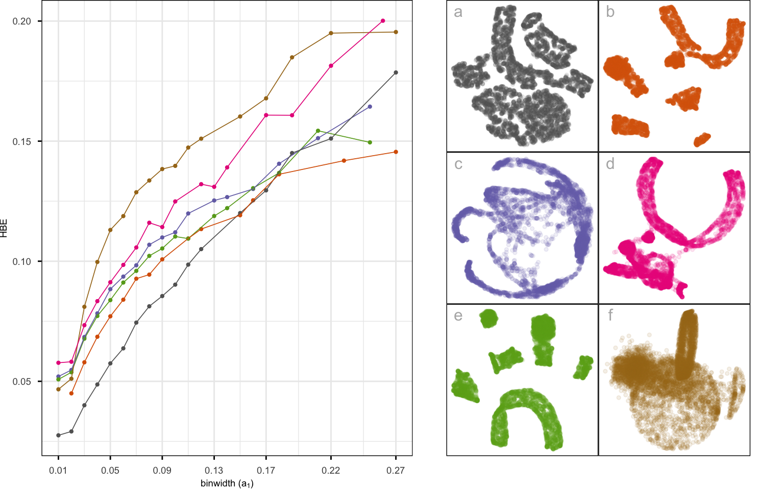
To assess their performance, we computed the hexbin error (HBE) between the observed high-dimensional data and the fitted values, defined as the high-dimensional mappings of the bin centroids (Gamage et al. 2025). A lower HBE indicates that the method better preserves the high-dimensional structure in its low-dimensional embedding.
As shown in Figure B.10, tSNE (Figure B.10 a) achieved the lowest HBE across bin widths (mostly small values), indicating strong preservation of local neighborhood structure. Its layout displays well-separated clusters with minimal inter-cluster distances, making it the most faithful representation of the underlying data structure. UMAP and PaCMAP (Figure B.10 b and e) produced moderately accurate embeddings, although the five clusters appear more well-separated, while PHATE (Figure B.10 c) shows nonlinear cluster structures irrespective of the original structure. Also, TriMAP (Figure B.10 d) has high HBE and shows three clusters with small distances. PCA (Figure B.10 f) failed to capture the nonlinear geometry, leading to the highest HBE.
Benchmarking clustering algorithms
To further evaluate the structure of the generated data, we benchmarked three clustering algorithms: k-means (Hartigan and Wong 1979), agglomerative hierarchical clustering with Ward’s linkage (Jr. 1963; Murtagh and Contreras 2012), and model-based clustering using Gaussian mixture models (Fraley and Raftery 2002; Scrucca et al. 2023) using the simulated dataset.
For model-based clustering, we use the "EII" covariance parameterization, which assumes spherical clusters with equal volume. This specification provides a constrained model that is broadly comparable to k-means clustering. While the Gaussian mixture framework allows more flexible covariance structures, these are not considered here, as the objective is to examine method behavior under a common baseline assumption rather than to optimize clustering performance.
Cluster validity statistics were computed using the cluster.stats() function from the fpc package (Hennig 2024). These indices capture different aspects of clustering quality, such as compactness and separation, and may not necessarily agree in their assessment of optimal cluster number. As discussed in Akhanli and Hennig (2020), such indices should be interpreted collectively rather than individually, and are most informative when used for comparative rather than absolute evaluation.
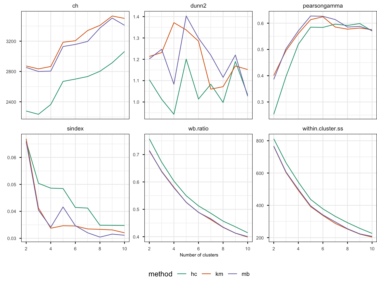
Figure 4.10 shows a selection of cluster metrics for 2-10 clusters for each of the methods, k-means, hierarchical, and model-based. As is typical, the suggestion of the best solution varies between cluster statistics. Although the metrics differ in their preferences, several show consistent support for a 4-5 cluster solution. Pearson gamma (pearsongamma) increases sharply up to five clusters before leveling off, Calinski–Harabasz index (ch) increases sharply from 4 to 5 clusters, and Dunn (dunn2) has a maximum at 5 for two methods and at 4 for k-means. All of these are interpreted as higher is better. With the other three, lower is better. WB ratio (wb.ratio) and within-cluster sum of squares (within.cluster.ss) steadily decline with the number of clusters, possibly elbowing around 5 clusters. The S-index (sindex) is optimized at 4 clusters for k-means, 3, 6, or 8 for hierarchical clustering, and 4 or 8 for model-based. Overall, k-means performs slightly better than the hierarchical and model-based clustering across most metrics and number of clusters.
Figure 4.11 shows the four- and five-cluster k-means solutions, with cluster id used to color the points. Neither solution captures the geometric nature of the true clusters, but they are both reasonable partitions of the data. To examine either one, it is best to subset to a single cluster to view in the tour. With each solution, the five original shapes are each split by the clustering. More than 5 clusters would be needed to better capture the original shapes.
Benchmarking of clustering methods typically requires multiple datasets, sensitivity analyses, and carefully controlled experimental designs (Mechelen et al. 2023). The present analysis is therefore intended as an illustrative case study demonstrating how standard clustering methods behave under complex geometric structure, rather than as a comprehensive benchmarking study.
4.5 Conclusion
The cardinalR package introduces a flexible framework for generating high-dimensional data structures with well-defined geometric properties. It addresses an important need in the evaluation of clustering, machine learning, and DR methods by enabling the construction of customized datasets with interpretable structures, noise characteristics, and clustering arrangements. In this way, cardinalR complements existing packages such as geozoo, snedata, and mlbench, while extending the scope to higher dimensions and more complex shapes.
The included structures cover a wide range of diagnostic settings. Branching shapes facilitate the study of continuity and topological preservation, the S-curve with a hole allows investigation of incomplete manifolds, and clustered spheres assess separability on curved surfaces. The Möbius strip introduces challenges from non-orientable geometry, while gridded cubes and pyrfrac test spatial regularity and clustering in sparse, non-convex regions.
These structures are designed to support not only algorithm diagnostics, but also teaching high-dimensional concepts, benchmarking reproducibility, and evaluating hyper-parameter sensitivity. By allowing users to adjust dimensionality, sample size, noise, and clustering properties, the package promotes transparent experimentation and comparative model evaluation. Together, these capabilities make cardinalR a versatile tool for generating interpretable, high-dimensional datasets that advance research, teaching, and evaluation of data-analytic methods.
Future extensions of cardinalR may include biologically inspired or application-driven data structures that would further broaden its utility in domains such as bioinformatics, forensic science, and spatial analysis.
4.6 Acknowledgements
The source material for this chapter, including the full datasets and figures, is available at https://github.com/JayaniLakshika/paper-cardinalR. This article is created using knitr (Xie 2015) and rmarkdown (Xie et al. 2018) in R with the rjtools::rjournal_article template. These R packages were used for this work: cli (Csárdi 2025), tibble (Müller and Wickham 2023), gtools (Warnes et al. 2023), dplyr (Wickham 2023), stats (R Core Team 2025), tidyr (Wickham et al. 2024), purrr (Wickham et al. 2025), mvtnorm (Genz and Bretz 2009), geozoo (Schloerke 2016), and MASS (Venables and Ripley 2002).